A view from Monte Carlo on the Third Ideal

Intending to underpin the relevance of “improvement of daily work”, I simulated a couple 100’000 years of development projects on my computer (487’462 years¹, to be exact) in an attempt to combine ideas from two books: The Unicorn Project by Gene Kim et al, and Fooled by randomness by Nicholas Nassim Taleb. This led me on a trajectory that was not exactly what I anticipated. But let’s start from the beginning.

The Unicorn Project and DevOps’ five Ideals

In The Unicorn Project, the five ideals of DevOps are explained to us by a savvy bartender named Eric. Those five ideals are:

1. Locality and Simplicity.
2. Focus, Flow, and Joy.
3. Improvement of Daily Work.
4. Psychological Safety.
5. Customer Focus.

The five ideals are nicely summarized in a blog post by Gene Kim.

These ideals are powerful as they are easy for anyone to accept. Not much debate about whether simplicity, or focus, or improvement of daily work are a good thing. At the same time, they are also generic enough so that many people can relate their behavior to them. Many an executive agrees to the first ideal, then goes ahead and complects the organization with the next reorg in the belief to increase the organization’s ability to perform.

Improvement of Daily Work

As for the third ideal, improvement of daily work, I sense that pretty much everyone acknowledges the value of continuous improvement, yet under the pressure of target dates and the subsequent “tyranny of the urgent”, many don’t live up to it. “Yes, improving our daily work is important, but first, we need to just jot out those features for the next release. We will have time afterwards.”

I felt that he ideal of “improvement of daily work” lends itself nicely to simulations. Maybe through a load of simulated projects, we can generate insights that help take the right decisions?

The Relevance of Alternative Realities

In the attempt to get a point across, especially if counter-intuitive to the addressee, as in the example of “we should focus less on feature development and more on productivity in oder to get our features done sooner”, we usually refrain to some success stories and/or concepts explained in books. Such stories are often rejected with arguments like “that’s not us”, “that’s not going to work around here”, “we’re a different type of industry/product/company”, you name it. As annoying such reactions are, they are not necessarily wrong, because our approach is inherently prone to the survivorship bias. When we sell a success story, we look at one particular case (or a set of cases) where a behavior was correlated to a positive outcome. We ignore the cases where the same behavior was correlated to a negative outcome – mainly because of the lack of their visibility. We only see the “survivors” – so we only analyze the “survivors”, and we tend to infer wrong causalities. That said, a fair bit of skepticism is in order. For mentioned addressees, a fictional story does not help either.

In Fooled by Randomness, Taleb explains the significant impact that randomness has on our lives, and how we’re being fooled by it. When assessing our reality, we often look at a given situation as a result of past events that were bound to happen. We take what happened for the only thing that could have happened, ignoring randomness. This is misleading – because what happened is, after all, just one out of may sequences of events that could have unfolded.

The aim of a monte carlo simulations is to generate alternative realities, those that could have unfolded just as well, but did not happen to. Looking at a broad range of possible realities, we can then gain a better understanding about (a) which kind of result is more likely to unfold, and (b) which of our assumptions have the biggest impact on the results.

Insights

So I got hooked on the idea of creating a monte carlo simulator to simulate product development realities and hopefully show that investing in improvement of daily work pays dividends based on factors that are irrespective of your domain, business, product, or whatever. And maybe we could even find a sweet spot for resource allocation…

If you are interested in more details about the simulations, the assumptions made, and the thinking behind them, Appendix A outlines that in some detail. The Appendix might help better understand the insights presented in this section.

We want to see whether the simulations support the third ideal as stated above – “improvement of daily work”. I simulated different strategies of investing resources, allocating 50% to 90% of resources to feature development (in steps of 10%) and distributing the rest to performance improvement and debt reduction (see table in the appendix).

My first hypothesis was that we would see an optimum of resource allocation to features. Allocating too much would result in less optimization and hence slower completion. Allocating too little would also get us away from the sweet spot, as we would use too few resources to actually profit from all the improvements.

So let’s see how the number of required iterations is distributed across the simulations with similar allocation to feature development. These box-charts display the mean value (average amount of iterations) as a green line. The blue box depicts the quartiles above and below the average, and the black T-shaped whiskers reflect the max and min values.

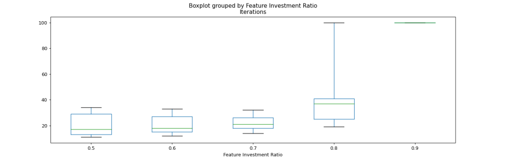
On a first sight, our hypothesis is confirmed by the mean values increasing with each step in what resembles a power-law distribution. There are few interesting observations here:

• In the simulated range, there seems to be no tipping point where the organization becomes slower due to a lack of focus on feature development. This, I find, is quite remarkable.
• While the number of required iterations increases steadily with increasing focus on feature development, the variability is smallest at 70% resources allocated to features. (except for 90%, where all simulated projects fail).
• We have failed projects only at 80% resources or above.

Next let’s see what the impact of the assumed interest rate on debt is. For this, we split up the graph further by interest rate and resource allocation to features.

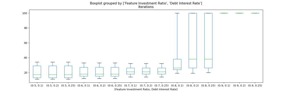
We can see that the interest rate only impacts scenarios with 80% resource allocation on features. The mean jumps as well as the upper quartile as the interest rate moves from 10% to 20%, while further increase to 25% seems to have no significant effect.

Let’s have a closer look at the projects with 80% resource allocation to features next. The histogram shows the distribution of required iterations, split by debt interest rates (0.1, 0.2, 0.25)

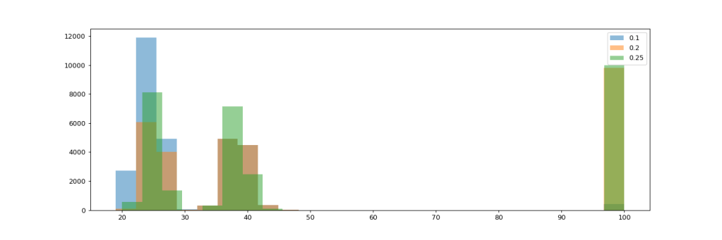
While I was expecting to find a continuum of iterations needed, we find that there’s actually two distinct group of projects: They either complete their scope within about 45 iterations, or they don’t finish within 100 – which allows the interpretation that they likely would not ever finish, irrespective of how long we let the project continue. This pattern is surprisingly stable across all levels of interest on debt.

We’re still aggregating three different strategies to resource allocation here (refer to table above). I suspected that the two distinct bumps in the above histogram might be related to the different levels of investment in Performance improvement, so let’s drill down further in the scenario with 20% debt interest and analyze the impact of investing in performance improvement. My hypothesis will be that higher invest in performance improvement will lead to fewer required iterations.

Now this hypothesis is obviously not confirmed by our data. While investing 10% of resources in performance improvement seems to yield greater gains than investing only 5%, 15% performs worst of the three. In fact, all of the failed attempts come from the strategy with the highest invest in performance. So what’s going on there?

We need to look into the trajectories of those failed projects to understand the situation better. The following graphs display the average values of team performance, remaining scope, and debt for each iteration. The colored areas display the respective min and max values. In addition, the histogram gives an overview on the remaining scope after the 100th iteration.

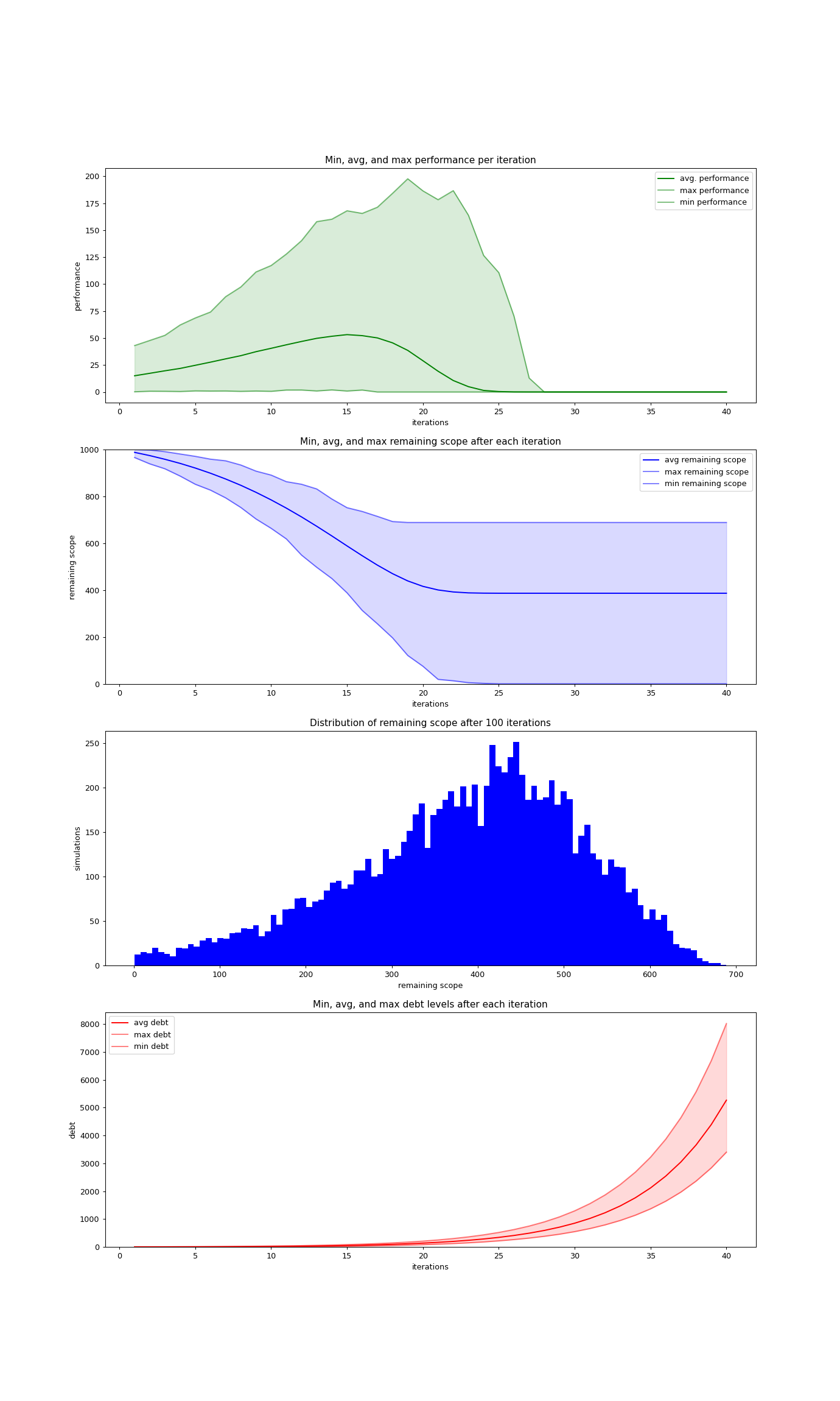
These graphs do tell an interesting story. It seems that for all the failed projects, the build-up of debt eventually impedes the team performance to the point where no progress on features is possible anymore, and debt continues to accumulate.

Conclusion

From the simulations and analysis done so far, I draw two conclusions:

1. The data seems to suggest that Improvement of Daily Work is certainly worth pursuing, and – counter to my expectations – I haven’t seen a “tipping point” where too much invest into improvement of daily work becomes counter-productive. All this, however, holds true only as long as you have your debt under control. Keeping quality in check (any aspect of it) is a precondition for the third ideal to play out.
2. There are more open than answered questions on this.

Open Questions

• How does the assumed impact that debt has on performance affect the results? And what would be a fair assumption to make about that impact? It could potentially change the trajectories significantly.
• How does the invest in productivity actually pay back in terms of improved capacity? The assumption taken for the simulation is pure gut-feeling and might impact the results if changed.
• Also, what would actually be a fair value to assume for the interest rate of debt?
• For any of those assumptions, do universal values exist at all? Is there a way to know up-front, so that we can optimize our investment strategies to such values? Or will we rather need entirely different strategies to allow dealing with the unknown and unknowable?
• The simulation uses mostly linear models – how accurate are they, and how does this (lack of) accuracy impact the results? E.g., can we assume that investing twice as much in performance improvement yields twice the return in terms of improvements? Isn’t the potential for improvement exhausted at some point, both when increasing the invest as well as over time? On the other hand, couldn’t investing more also unleash exponential improvements that were otherwise never possible?

The list goes on and on, and I sincerely hope to be able to run more simulations and come up with more insights over time.

As for now, the take-hope message is limited to this:

1. Keep your debt in check
2. Pursue improvement of daily work
3. You likely overestimate the impact of investing into features for your overall progress.

Appendix A – Simulating Product Development

First of all, I decided I would simulate endeavors with a set of starting conditions:

• In every endeavor, a product backlog of 1’000 story points needs to be “worked down”. Since we don’t assign any actual scope to the number, for the sake of the simulation it is irrelevant how stable that backlog is content-wise. Also it would not impact the simulation if the backlog would be built up continuously over time, assuming that the team does not run out of work throughout the simulation.
• In every endeavor, the Team starts with an initial capacity of 20 story points per iteration.
• We will simulate a max of 100 iterations for each endeavor. If the product backlog is not fully “worked down” by then, the project’s considered failed and the simulation is stopped. With a backlog of 1’000 story points and a capacity of 20 story points per iteration, the backlog would be expected to be done after 50 iterations.

Note that the actual scale of the simulation is irrelevant – whether it’s a single team with a product (fairly small story points), or a large, multi-team organization building a huge product (fairly large story points) makes no difference.

Further note that the iteration can account for a large variety of setups. For an organization using Scrum, tit might be a sprint of whatever length. However, it might just as well reflect product increments in a SAFe environment, or a regular cadence in which we observe and measure a system based on continuous flow (Kanban).

Capacity, Productivity, Debt, and Features

Capacity vs. Productivity

Capacity in our simulation means the amount of story points that a team would be expected to work down during an iteration under expected circumstances. Most scrum teams, for example, assess their team’s capacity for a sprint based on recent performance, absences, etc.

Reality rarely follows the plan. Unplanned absences but also under- or over-estimated work items impact the teams ability to deliver. In the simulation, we refer to the amount of story points that a team is actually able to deliver as its productivity.

This is where Monte Carlo enters the picture: By subjecting the theoretical capacity to a degree of randomness (called “success factor”) in each iteration, we get the simulated productivity.

As the legend goes, a team that does not invest in its productivity will eventually, by laws of thermodynamics and due to entropy, reduce it’s capacity to deliver. I don’t know of any research about this (if you do, please leave a link in the comments!), but the legend is so popular that the simulation accounts for this, too.

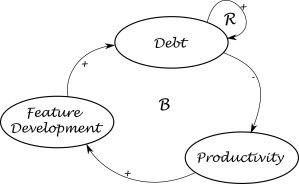
Dealing with Debt

From a qualitative perspective, we can say that:

• When we build features, inevitably, we will build up some debt. Technical debt, but also quality debt. In our simulation, all debt is combined in a single value, and we track it in the currency of story points for reasons of simplicity.
• Debt leads to more debt – an issue that easy to fix right away will be much more difficult to resolve a few months down the line. Also, technical debt that we decide to work around instead of fixing will be more severe afterwards, because to fix it, we will also need to fix the workaround eventually.
• Debt reduces productivity – the more debt that’s in the system and that needs to be (a) managed and (b) worked around, the more difficult it is for the team to get stuff done. The simulation accounts for this by having debt impact the capacity for every iteration.

Simulating different Strategies

The simulation allows to define how the productivity of a team is invested in three different areas:

• Feature Development: The share of the team’s productivity that goes into reducing the feature backlog.
• Debt Reduction: The share of the team’s productivity that goes into reducing already built-up debt. This represents reducing technical debt, documentation debt, but also quality debt like fixing bugs.
• Performance Improvement: The share of the team’s productivity that is invested in measures to drive up the team’s capacity in the future. This reflects work like automating repetitive tasks, creating or shortening feedback loops, investing in continuous delivery capabilities, measures to improve collaboration, etc.

Note some limitations in the simulation:

1. How the productivity of a team is invested across these three categories remains constant throughout the simulation. For the sake of simplicity, we derive the productivity from the capacity as described above, then split the productivity according to the defined strategy and apply it to calculate the iteration’s outcomes.
2. As a consequence of (1), the variability is limited to the “success” of the sprint. Some sprints might deliver 0 results, other might result in a firework of stuff done.
3. Also as a consequence of (1), when the capacity assigned to debt reduction exceeds the actual debt, the excess capacity is lost for the iteration. This fact penalizes high invest in debt reduction.
4. Investment in performance improvements affects the capacity of the team for upcoming iterations.
5. To avoid dealing with decimal places in remaining scope values, the simulation always rounds capacity to a natural number. The simulation, on the other hand, does not account for the usual Fibonacci-like series applied with story points.

So far, the simulation covers 13 different strategies, a combination of 50% to 90% of capacity invested in feature development, and the rest either in favor of debt reduction or performance improvement, or balanced between the two. For each investment strategy, the simulation runs 10’000 projects. The simulation stops when the backlog becomes empty (i.e., 0 story points), or after 100 iterations.

Feature Development	Debt Reduction	Performance Improvement
50%	40%	10%
50%	25%	25%
50%	10%	40%
60%	30%	10%
60%	20%	20%
60%	10%	30%
70%	20%	10%
70%	15%	15%
70%	10%	20%
80%	5%	15%
80%	10%	10%
80%	15%	5%
90%	5%	5%

A word on the randomness

In order to make the different strategies more comparable, I seed the random generator identically for each strategy, so that each simulated set of projects is subjected to the same set of “realities”.

Assumptions

The simulation necessarily builds on a set of assumptions that might significantly impact the results. Among them:

• Debt Interest Rate: How much does the load of existing debt grow if it is not tackled? I ran simulations with three different rates:
  • 10% – while 10% seems a lot, it effectively means a duplication after ~7 iterations. That would mean a bug that an be fixed in half a day if we just tackle it right away, will need require a day of work 7 iterations later. Without further data at hand, my gut-feeling is that this is a rather optimistic assumption.
  • 20% – means a duplication every 4 iterations, so in this case, some clean-up or bug-fix that we postpone might be twice as much work to get rid of after 4 iterations.
  • 25% – means a duplication every 3 iterations, which feels rather pessimistic to me.
• Debt from new features : How much is the ratio of debt created from new features? For now, I worked with the assumption of 10%.
• Debt impact on productivity: How does debt affect the teams capacity/productivity? Lacking real-life information, the simulation uses a shortcut here: The ratio of invest impacts the performance directly. If you invest 100% in performance improvement, then the performance doubles every iteration (well, almost, because of the drain). This is clearly a very simplistic way of modeling this.
• Performance drain: How much does the performance drain if the team does not pay attention to it? I simulated all runs with a drain of 1% per iteration, which effectively means the performance would be reduced to half its value after 69 iterations.

---

¹ 12’708’831 simulated iterations, assuming 2 weeks per iteration results in 25’417’662 weeks or 487’462 years.

Title photo by Anna Shvets on Pexels.com